Note
Go to the end to download the full example code.
Train, convert and predict with ONNX Runtime#
This example demonstrates an end to end scenario starting with the training of a machine learned model to its use in its converted from.
Train a logistic regression#
The first step consists in retrieving the iris dataset.
Then we fit a model.
We compute the prediction on the test set and we show the confusion matrix.
[[12  0  0]
 [ 0 13  0]
 [ 0  2 11]]
Conversion to ONNX format#
We use module sklearn-onnx to convert the model into ONNX format.
from skl2onnx import convert_sklearn  # noqa: E402
from skl2onnx.common.data_types import FloatTensorType  # noqa: E402

initial_type = [("float_input", FloatTensorType([None, 4]))]
onx = convert_sklearn(clr, initial_types=initial_type)
with open("logreg_iris.onnx", "wb") as f:
    f.write(onx.SerializeToString())
We load the model with ONNX Runtime and look at its input and output.
import onnxruntime as rt  # noqa: E402

sess = rt.InferenceSession("logreg_iris.onnx", providers=rt.get_available_providers())

print(f"input name='{sess.get_inputs()[0].name}' and shape={sess.get_inputs()[0].shape}")
print(f"output name='{sess.get_outputs()[0].name}' and shape={sess.get_outputs()[0].shape}")
input name='float_input' and shape=[None, 4]
output name='output_label' and shape=[None]
We compute the predictions.
input_name = sess.get_inputs()[0].name
label_name = sess.get_outputs()[0].name

import numpy  # noqa: E402

pred_onx = sess.run([label_name], {input_name: X_test.astype(numpy.float32)})[0]
print(confusion_matrix(pred, pred_onx))
[[12  0  0]
 [ 0 15  0]
 [ 0  0 11]]
The prediction are perfectly identical.
Probabilities#
Probabilities are needed to compute other relevant metrics such as the ROC Curve. Let’s see how to get them first with scikit-learn.
prob_sklearn = clr.predict_proba(X_test)
print(prob_sklearn[:3])
[[9.83067256e-01 1.69326850e-02 5.91040175e-08]
 [2.02946333e-03 4.42657924e-01 5.55312612e-01]
 [1.73767942e-07 9.82234790e-03 9.90177478e-01]]
And then with ONNX Runtime. The probabilities appear to be
prob_name = sess.get_outputs()[1].name
prob_rt = sess.run([prob_name], {input_name: X_test.astype(numpy.float32)})[0]

import pprint  # noqa: E402

pprint.pprint(prob_rt[0:3])
[{0: 0.9830672144889832, 1: 0.016932697966694832, 2: 5.910407097076131e-08},
 {0: 0.0020294631831347942, 1: 0.4426578879356384, 2: 0.5553126931190491},
 {0: 1.7376801508817152e-07, 1: 0.009822347201406956, 2: 0.9901774525642395}]
Let’s benchmark.
from timeit import Timer  # noqa: E402


def speed(inst, number=5, repeat=10):
    timer = Timer(inst, globals=globals())
    raw = numpy.array(timer.repeat(repeat, number=number))
    ave = raw.sum() / len(raw) / number
    mi, ma = raw.min() / number, raw.max() / number
    print(f"Average {ave:1.3g} min={mi:1.3g} max={ma:1.3g}")
    return ave


print("Execution time for clr.predict")
speed("clr.predict(X_test)")

print("Execution time for ONNX Runtime")
speed("sess.run([label_name], {input_name: X_test.astype(numpy.float32)})[0]")
Execution time for clr.predict
Average 5.4e-05 min=4.82e-05 max=8.02e-05
Execution time for ONNX Runtime
Average 1.83e-05 min=1.67e-05 max=2.72e-05

1.8263659999320225e-05
Let’s benchmark a scenario similar to what a webservice experiences: the model has to do one prediction at a time as opposed to a batch of prediction.
def loop(X_test, fct, n=None):
    nrow = X_test.shape[0]
    if n is None:
        n = nrow
    for i in range(n):
        im = i % nrow
        fct(X_test[im : im + 1])


print("Execution time for clr.predict")
speed("loop(X_test, clr.predict, 50)")


def sess_predict(x):
    return sess.run([label_name], {input_name: x.astype(numpy.float32)})[0]


print("Execution time for sess_predict")
speed("loop(X_test, sess_predict, 50)")
Execution time for clr.predict
Average 0.00191 min=0.0016 max=0.00234
Execution time for sess_predict
Average 0.000307 min=0.000303 max=0.000334

0.00030683602000181054
Let’s do the same for the probabilities.
print("Execution time for predict_proba")
speed("loop(X_test, clr.predict_proba, 50)")


def sess_predict_proba(x):
    return sess.run([prob_name], {input_name: x.astype(numpy.float32)})[0]


print("Execution time for sess_predict_proba")
speed("loop(X_test, sess_predict_proba, 50)")
Execution time for predict_proba
Average 0.00221 min=0.00218 max=0.00228
Execution time for sess_predict_proba
Average 0.00031 min=0.000305 max=0.000335

0.00030961111999886274
This second comparison is better as ONNX Runtime, in this experience, computes the label and the probabilities in every case.
Benchmark with RandomForest#
We first train and save a model in ONNX format.
from sklearn.ensemble import RandomForestClassifier  # noqa: E402

rf = RandomForestClassifier(n_estimators=10)
rf.fit(X_train, y_train)

initial_type = [("float_input", FloatTensorType([1, 4]))]
onx = convert_sklearn(rf, initial_types=initial_type)
with open("rf_iris.onnx", "wb") as f:
    f.write(onx.SerializeToString())
We compare.
sess = rt.InferenceSession("rf_iris.onnx", providers=rt.get_available_providers())


def sess_predict_proba_rf(x):
    return sess.run([prob_name], {input_name: x.astype(numpy.float32)})[0]


print("Execution time for predict_proba")
speed("loop(X_test, rf.predict_proba, 50)")

print("Execution time for sess_predict_proba")
speed("loop(X_test, sess_predict_proba_rf, 50)")
Execution time for predict_proba
Average 0.0162 min=0.0159 max=0.0176
Execution time for sess_predict_proba
Average 0.000302 min=0.000295 max=0.000334

0.0003015268800004378
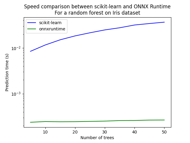
Let’s see with different number of trees.
measures = []

for n_trees in range(5, 51, 5):
    print(n_trees)
    rf = RandomForestClassifier(n_estimators=n_trees)
    rf.fit(X_train, y_train)
    initial_type = [("float_input", FloatTensorType([1, 4]))]
    onx = convert_sklearn(rf, initial_types=initial_type)
    with open(f"rf_iris_{n_trees}.onnx", "wb") as f:
        f.write(onx.SerializeToString())
    sess = rt.InferenceSession(f"rf_iris_{n_trees}.onnx", providers=rt.get_available_providers())

    def sess_predict_proba_loop(x):
        return sess.run([prob_name], {input_name: x.astype(numpy.float32)})[0]  # noqa: B023

    tsk = speed("loop(X_test, rf.predict_proba, 25)", number=5, repeat=4)
    trt = speed("loop(X_test, sess_predict_proba_loop, 25)", number=5, repeat=4)
    measures.append({"n_trees": n_trees, "sklearn": tsk, "rt": trt})

from pandas import DataFrame  # noqa: E402

df = DataFrame(measures)
ax = df.plot(x="n_trees", y="sklearn", label="scikit-learn", c="blue", logy=True)
df.plot(x="n_trees", y="rt", label="onnxruntime", ax=ax, c="green", logy=True)
ax.set_xlabel("Number of trees")
ax.set_ylabel("Prediction time (s)")
ax.set_title("Speed comparison between scikit-learn and ONNX Runtime\nFor a random forest on Iris dataset")
ax.legend()
5
Average 0.00591 min=0.0055 max=0.00698
Average 0.000157 min=0.000148 max=0.000178
10
Average 0.0084 min=0.00801 max=0.00946
Average 0.000157 min=0.000147 max=0.000182
15
Average 0.0113 min=0.0107 max=0.0121
Average 0.000167 min=0.000156 max=0.000183
20
Average 0.013 min=0.0128 max=0.0134
Average 0.000159 min=0.00015 max=0.00018
25
Average 0.0156 min=0.0153 max=0.0167
Average 0.000162 min=0.000154 max=0.000185
30
Average 0.0181 min=0.0176 max=0.0191
Average 0.000163 min=0.000155 max=0.000187
35
Average 0.0204 min=0.0199 max=0.0214
Average 0.000167 min=0.000158 max=0.000191
40
Average 0.0228 min=0.0223 max=0.0237
Average 0.000168 min=0.000158 max=0.000192
45
Average 0.0253 min=0.0249 max=0.0263
Average 0.000168 min=0.00016 max=0.000192
50
Average 0.0278 min=0.0275 max=0.0285
Average 0.000172 min=0.000161 max=0.000194

<matplotlib.legend.Legend object at 0x7b9d20f7d000>
Total running time of the script: (0 minutes 5.015 seconds)